Whether you are fairly new to data science techniques or even a seasoned veteran, interpreting results from a machine learning algorithm can be a trying experience. The challenge is making sense of the output of a given model. Does that output tell you how well the model performed against the data you used to create and "train" it (i.e., training data)? Does the output give you a good read on how well your model performed against new/unknown inputs (i.e., test data)?
There are often many indicators and they can often lead to differing interpretations. The biggest problem some of us have is trying to remember what all the different indicators mean. Some indicators refer to characteristics of the model, while others refer to characteristics of the underlying data.
In this post, we will examine some of these indicators to see if the data is appropriate to a model. Why do we care about the characteristics of the data? What's wrong with just stuffing the data into our algorithm and seeing what comes out?
The problem is that there are literally hundreds of different machine learning algorithms designed to exploit certain tendencies in the underlying data. In the same way different weather might call for different outfits, different patterns in your data may call for different algorithms for model building.
Certain models make assumptions about the data. These assumptions are key to knowing whether a particular technique is suitable for analysis. One commonly used technique in Python is Linear Regression. Despite its relatively simple mathematical foundation, linear regression is a surprisingly good technique and often a useful first choice in modeling. However, linear regression works best with a certain class of data. It is then incumbent upon us to ensure the data meets the required class criteria.
In this particular case, we'll use the Ordinary Least Squares (OLS)method that comes with the statsmodel.api module. If you have installed the Anaconda package (https://www.anaconda.com/download/), it will be included. Otherwise, you can obtain this module using the pip command:
pip install -U statsmodels
In Windows, you can run pip from the command prompt:
We are going to explore the mtcars dataset, a small, simple dataset containing observations of various makes and models.
You can download the mtcars.csv here.
(https://gist.github.com/seankross/a412dfbd88b3db70b74b)
I'll use this Python snippet to generate the results:
import pandas aspd
importstatsmodels.api assm
## Setting Working directory
importos
path = "C:\\Temp"
os.chdir(path)
## load mtcars
mtcars = pd.read_csv(".\\mtcars.csv")
## Linear Regression with One predictor
## Fit regression model
mtcars["constant"]= 1
## create an artificial value to add a dimension/independent variable
## this takes the form of a constant term so that we fit the intercept
## of our linear model
## we can then use the intercept-only model as our null hypothesis
X = mtcars.loc[:,["constant","am"]]
## mpg is our dependent variable
Y = mtcars.mpg
# create the model
mod1res = sm.OLS(Y, X).fit()
## Inspect the results
print(mod1res.summary())
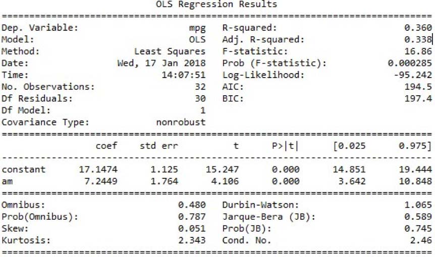
Assuming everything works, the last line of code will generate a summary that looks like this:
The section we are interested in is at the bottom. The summary provides several measures to give you an idea of the data distribution and behavior. From here we can see if the data has the correct characteristics to give us confidence in the resulting model. We aren't testing the data, we are just looking at the model's interpretation of the data. If the data is good for modeling, then our residuals will have certain characteristics. These characteristics are:
The data is "linear". That is, the dependent variable is a linear function of independent variables and an error term e, and is largely dependent on characteristics 2-4. Think of the equation of a line in two dimensions: y = mx + b + e. yis the dependent or "response" variable, xis the input, mis the dimensional coefficient and bis the intercept (when x = 0). We can easily extend this "line" to higher dimensions by adding more inputs and coefficients, creating a hyperplane with the following form: y = a1x1+ a2x2+ … + anxn
Errors are normally distributed across the data. In other words, if you plotted the errors on a graph, they should take on the traditional bell-curve or Gaussian shape.
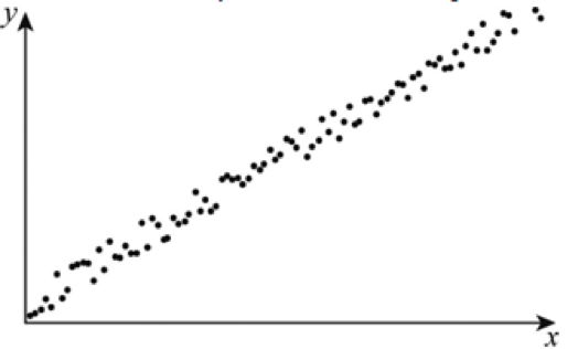
There is "homoscedasticity". This means that the variance of the errors is consistent across the entire dataset. We want to avoid situations where the error rate grows in a particular direction. This is homoscedastic:
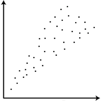
This is not:
Note that in the first graph variance between the high and low points at any given X value are roughly the same. In the second graph, as X grows, so does the variance.
The independent variables are actually independent and not collinear. We want to ensure independence between all of our inputs, otherwise our inputs will affect each other, instead of our response.
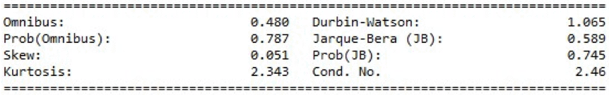
The results of the linear regression model run above are listed at the bottom of the output and specifically address those characteristics. Here's another look:
Let's look at each of the values listed:
Omnibus/Prob(Omnibus) – a test of the skewness and kurtosis of the residual (characteristic #2). We hope to see a value close to zero which would indicate normalcy. The Prob (Omnibus) performs a statistical test indicating the probability that the residuals are normally distributed. We hope to see something close to 1 here. In this case Omnibus is relatively low and the Prob (Omnibus) is relatively high so the data is somewhat normal, but not altogether ideal. A linear regression approach would probably be better than random guessing but likely not as good as a nonlinear approach.
Skew – a measure of data symmetry. We want to see something close to zero, indicating the residual distribution is normal. Note that this value also drives the Omnibus. This result has a small, and therefore good, skew.
Kurtosis – a measure of "peakiness", or curvature of the data. Higher peaks lead to greater Kurtosis. Greater Kurtosis can be interpreted as a tighter clustering of residuals around zero, implying a better model with few outliers.
Durbin-Watson – tests for homoscedasticity (characteristic #3). We hope to have a value between 1 and 2. In this case, the data is close, but within limits.
Jarque-Bera (JB)/Prob(JB) – like the Omnibus test in that it tests both skew and kurtosis. We hope to see in this test a confirmation of the Omnibus test. In this case we do.
Condition Number – This test measures the sensitivity of a function's output as compared to its input (characteristic #4). When we have multicollinearity, we can expect much higher fluctuations to small changes in the data, hence, we hope to see a relatively small number, something below 30. In this case we are well below 30, which we would expect given our model only has two variables and one is a constant.
In looking at the data we see an "OK" (though not great) set of characteristics. This would indicate that the OLS approach has some validity, but we can probably do better with a nonlinear model.
Data "Science" is somewhat of a misnomer because there is a great deal of "art" involved in creating the right model. Understanding how your data "behaves" is a solid first step in that direction and can often make the difference between a good model and a much better one.
Kevin McCarty is a freelance Data Scientist and Trainer. He teaches data analytics and data science to government, military, and businesses in the US and internationally.
Kevin has a PhD in computer science and is a data scientist consultant and Microsoft Certified Trainer for .NET, Machine Learning and the SQL Server stack. He also trains and consults on Python, R and Tableau. Kevin has taught for Accelebrate all over the US and in Africa.