Support Vector Machine Advanced Techniques
We offer private, customized training for 3 or more people at your site or online.
In part 2 of this tutorial series, we set up a simple support vector classifier to classify handwriting samples as specific digits. In this tutorial, we will expand the code to load data with Pandas, save/load the trained model, and explore how to determine the best hyperparameters for the support vector classifier.
Using a Support Vector Machine
Training a Support Vector Machine (SVM) is only one part of machine learning. Before a model can be used in the real world, the training/testing data must be prepared and the model (predictor function) must be trained. Finding and preparing data is probably the most time-consuming part of machine learning, as there are many data sources to consider and different types of preparatory analysis to perform first.
Two useful tools in the Python world for performing such data munging tasks are NumPy and Pandas. NumPy is great for performing numerical analysis, and Pandas (which utilizes NumPy and database libraries such as SQLAlchemy) is useful for loading and preparing data.
To save and load trained models, scikit-learn comes with a JobLib. JobLib uses Python's serialization process to serialize the trained models that typically contain a lot of NumPy data.
An important part of training an SVM is to select the best hyperparameters. Usually, this is done by training and testing the model repeatedly with different hyperparameters.
Step 1. Loading Data with Pandas
Performing machine learning requires plenty of data that can be loaded from data sources such as relational databases, document storage, CSV files, etc. A very popular Python library for loading, preparing, and analyzing data is the Pandas library. Coupled with other libraries, such as SQLAlchemy and NumPY, Pandas has amazing data access and analysis abilities. Fortunately, the datasets provided by Sci-Kit Learn do not require loading and preparing, however, real-world datasets will. We will explore how to load some custom testing data using Pandas.
Step 1.1 Make a copy of the current "?Predict a Number and Display It" notebook from the previous tutorial using the "File" menu's "Make a Copy" option. Rename the notebook "Load a Number with Pandas and Predict a Number." If you did not complete the previous tutorial, use the example from the https://github.com/t4d-accelebrate-tutorials/ml-tutorial.
In this step, we will load some digit data from a CSV file with Pandas and then predict (classify) the digit with our support vector classifier.
Step 1.2 Using Jupyter Notebooks, create a new text file named "digits.csv" in the project folder. Copy and paste the following text into the file:
0,0,0,0,16,0,0,0,0,0,0,0,16,0,0,0,0,0,0,0,16,0,0,0,0,0,0,0,16,0,0,0, 0,0,0,0,16,0,0,0,0,0,0,0,16,0,0,0,0,0,0,0,16,0,0,0,0,0,0,0,16,0,0,0
Save the file and close the tab.
Step 1.3 Next open the "Load a Number with Pandas and Predict a Number" notebook. The Pandas package was installed in the first tutorial when setting up the project environment with Conda. Update the code at the top of the notebook cell to import the pandas module:
from sklearn import datasets, svm
import matplotlib.pyplot as plt
import pandas as pd
Step 1.4 Replace the hard-coded sample number assignment code:
sample_number = [
  [ 0.,  0.,  0.,  0.,  16.,  0.,  0.,  0. ],
  [ 0.,  0.,  0.,  0.,  16.,  0.,  0.,  0. ],
  [ 0.,  0.,  0.,  0.,  16.,  0.,  0.,  0. ],
  [ 0.,  0.,  0.,  0.,  16.,  0.,  0.,  0. ],
  [ 0.,  0.,  0.,  0.,  16.,  0.,  0.,  0. ],
  [ 0.,  0.,  0.,  0.,  16.,  0.,  0.,  0. ],
  [ 0.,  0.,  0.,  0.,  16.,  0.,  0.,  0. ],
  [ 0.,  0.,  0.,  0.,  16.,  0.,  0.,  0. ],
]
with the following code:
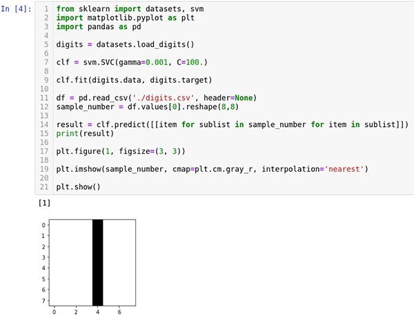
df = pd.read_csv('./digits.csv', header=None)
sample_number = df.values[0].reshape(8,8)
Pandas provide excellent CSV reading and writing capabilities. There are numerous options such as indicating whether the data being read in has a header. With the digit attributes loaded, the data needs to be reshaped into an 8x8 NumPy array structure so it can be understood by the list comprehension.
Step 1.5 Run the cell now and verify the prediction results. The notebook should look like this:

Step 2. Saving and Re-Loading the Model
The result of training a support vector classifier is a trained model that can be used repeatedly. To reuse the model, there needs to be a mechanism for saving the model so it can be reloaded in the future to be used again.
Step 2.1 Make a copy of the "Load a Number with Pandas and Predict a Number" notebook from the previous step and rename it to "?Save and Load the Predict a Number Model."
Step 2.2 Update the imports at the top of the notebook cell to import joblib so that models can be saved and loaded again:
from sklearn import datasets, svm
from sklearn.externals import joblib
import matplotlib.pyplot as plt
import pandas as pd
Step 2.3 To save the model, add the following code immediately after the call to the predict method:
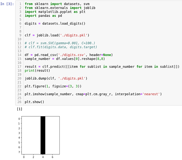
joblib.dump(clf, './digits.pkl')
Step 2.4 Run the notebook cell and there will be a new file named "digits.pkl". It is a binary file, so there is nothing to inspect, but the model has been saved.
Step 2.5 To load the model, add this code immediately before the call to the svm.SVC:
clf = joblib.load('./digits.pkl')
Step 2.6 Comment out the following two lines of code:
?# clf = svm.SVC(gamma=0.001, C=100.)
# clf.fit(digits.data, digits.target)
Step 2.7 Run the notebook cell. The output should be the same as earlier. The notebook should look like this:

Step 3. Optimizing the Hyperparameters
In the second tutorial, two arguments were passed into the support vector classifier to configure two important hyperparameters of the classifier. In fact, had those hyperparameters not been specified, the classifier would not have worked as well as it did. A hyperparameter is a parameter used to create the model (predictor function), whereas a normal parameter is the parameter passed into the model (predictor function) to generate a result. To help us configure the classifier (select the right hyperparameters), scikit-learn provides the Grid Search API to help find the optimal hyperparameters based on the training set. The overall operation is helpful, but can be time-consuming to run.
For this tutorial, the RBF (radial basis function) is used for the kernel function. There are several kernel functions from which to choose and even a custom kernel function can be coded. The other built-in kernel options include the linear, polynomial, and sigmoid functions. The RBF function is the default (and preferred) because it is faster than the other kernels and it can map and approximate almost any nonlinear function.
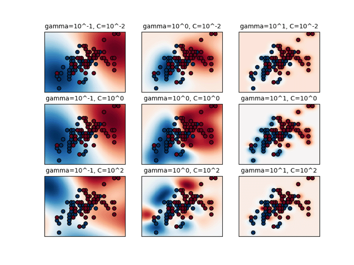
Using the RBF kernel, the SVM draws a bubble (representing influence) around each support vector (the vectors near the boundary). The bubbles (amount of influence) are expanded and contracted until they reach each other to form a decision surface (the boundary between classifications). The expansion and contraction are driven by the gamma hyperparameter value. A high gamma value reduces the influence (size of the bubble), and a low gamma value increases the influence (size of the bubble). The gamma value is inverse to the radius of the bubble (influence) surrounding the support vector.
A lower gamma results in smoother decision surface curves which may result in a less accurate classifier. A higher gamma fits the training data more closely but can result in over-fitting. One great feature of the RBF approach is that it adapts to the data very well, which reduces bias. The linear kernel does not support curves, and the sigmoid and polynomial kernel functions are not as adaptable thereby increasing bias.

Source: http://scikit-learn.org/stable/_images/sphx_glr_plot_rbf_parameters_001.png
The second hyperparameter needed is C. The C hyperparameter determines the amount of misclassification in return for a smoother decision surface. The value of C increases or decreases the number of support vectors utilized to calculate the decision surface. A low C results in a smoother surface but will have higher misclassification rates. A high C results in a curvier surface that can over-fit the training data.
To summarize, the gamma and C hyperparameters affect the decision surface in similar ways but through different approaches. The gamma sets the size of influence for each support vector and the C value helps determine the number of support vectors selected to create the decision surface. A higher gamma or C makes the classifier more accurate but could result in over-fitting. A low gamma or C makes the classifier less accurate but avoids over-fitting the training data. Generally, a balance is struck between the gamma value and the C value to create a smooth, accurate decision surface without over-fitting. Selecting the right gamma and C values can be done through grid search analysis, which is covered in the forthcoming third tutorial.
Once an SVM has been trained, it can be used as a predictor function to predict new results based upon new inputs.
Step 3.1 Make a copy of the "?Save and Load the Predict a Number Model" notebook from the previous step and rename it to "?Optimize the Hyperparameters for the Predict a Number Model."
Step 3.2 Update the imports to include the GridSearchCV and the numpy modules:
from sklearn import datasets, svm
from sklearn.externals import joblib
from sklearn.grid_search import GridSearchCV
import matplotlib.pyplot as plt
import pandas as pd
import numpy as np
Step 3.3 Delete all the code that follows the loading of the digits data. Do NOT delete the digits loading code.
To search for the best hyperparameters, the learning algorithm must be configured. In this case, we are searching for the best hyperparameters for the RBF kernel, so the kernel will be initialized to "RBF." Also, to ensure the same random occurs with each run, the random_state will be initialized to "101."
Step 3.4 Following the digits loading code, add the following line of code to initialize the support vector classifier:
clf = svm.SVC(kernel='rbf', random_state=101)

The GridSearchCV will use a pre-defined search space to look for the best hyperparameters.
Searching for the best values is CPU and time intensive so a reasonable search space should be specified.
In this case, the search is being limited to the "RBF" kernel, but the possible values of C and gamma will be explored.
Step 3.5 Add the following code to define the hyperparameter search space.
# both of these option arrays could be written with np.logspace
C_options = np.array([0.001, 0.01, 0.1, 1, 10, 100, 1000])
gamma_options = np.array([0.001, 0.01, 0.1, 0.0, 10.0, 100.0, 1000])
hyperparameter_search_space = [{'kernel': ['rbf'],
            'C': C_options,
            'gamma': gamma_options}]
With the hyperparameter search space defined, the GridSearchCV now needs to be configured and instantiated. In addition to the support vector classifier and the hyperparameter search space, the GridSearchCV needs to know how many folds to divide the training data into to perform cross-validation. This is specified with the cv parameter.
kFolds
The cv parameter specifies the number of kFolds (explained in detail below) to use for cross-validation. When training a model, the dataset is divided into training data and test data. Models are trained with training data and tested with the test data. With each iteration of testing, hyperparameters are adjusted, training is repeated, and the updated model is tested. While this is a good approach, the inevitable result with enough iterations of adjusting hyperparameters is that "knowledge" of the test dataset creeps into the values set for the hyperparameters. This creeping of "knowledge" results in the model becoming over-fitted to the test data.
Over-fitting either the training data or test data is undesirable. To solve this problem, a third set of data can be extracted from the overall dataset, called the validation set. The validation set is used in the iterative process of tweaking hyperparameters and finally, when all is good, the test set is used. This additional layer prevents over-fitting the test data. The problem with this approach is that the segmenting of the data into three sets greatly reduces the amount of data available for training.
An alternative approach, named kFolds, is to divide the training data (the test data is not included) into a number (k) of folds. When training, k – 1 folds are used for training and the remaining fold is used for cross-validation. The process is repeated where the fold used for cross-validation is used for training, and another fold is used for cross-validation. Averages are computed for each iteration, resulting in hyperparameters that do not over-fit the training data. Additionally, kFolds cross-validates data and experiences a minimal knowledge leak from the test data. A higher number of folds increases training time significantly, but decreases the chance of over-fitting.
Step 3.6 Create a new grid search object using the support vector classifier, hyperparameter search space and the number of folds.
gridsearch = GridSearchCV(clf,
             param_grid=hyperparameter_search_space,
             cv=10)
Step 3.7 The fit method is invoked with the training data (inputs and target classification). Add the following code to perform the fit:
gridsearch.fit(digits.data[:-1], digits.target[:-1])
Step 3.8 Retrieve the cross-validation and test scores from the grid search. For the test score, the final data point in the digits dataset is used. Add the following code to retrieve score values:
cv_performance = gridsearch.best_score_
test_performance = gridsearch.score(digits.data[-1:], digits.target[-
1:])
Step 3.9 Add the following code to output the score values:
?print('Best parameter: {}'.format(str(gridsearch.best_params_)))
print('Cross-validation accuracy score: {0:0.3f}'.format(cv_performance))
print('Test accuracy score: {0:0.3f}'.format(test_performance))
Run the notebook cell. The first time you run it, you may receive a deprecation warning. It can be safely ignored. Rerun the notebook cell and wait several minutes (it takes a while).
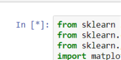
It's easy to know a cell is running. If you look in the center of the square brackets next to the cell and see an asterisk, the cell is running.

When the cell completes, the asterisk will change to a number. The number increments on each run of the cell.

The results of the operation are:

The results of the grid search are the best hyperparameters in the search space that can be used to configure the support vector classifier. The cross-validation score and the test score show the accuracy of those hyperparameters when running the search. The higher the numbers, the better.
Conclusion
Machine learning is an exciting, popular and growing field of software development. Combining the power of subject matter expertise, mathematics and programming to predict the future is changing how businesses operate, streamlining the lives of everyday people and changing how software impacts the world.
Resources
The following web sites and books were consulted in the creation of this tutorial series:

