SSAS 2008: BIDS and Data Cube Tutorial

• Exercise Files
• Sample DB from CodePlex

• Understanding Analysis Services
• Introducing BIDS
• Creating a Data Cube
• Exploring a Data Cube

• AdventureWorksCube1.zip
• AdventureWorksCube2.zip

• SSRS 2012: Enhanced Report Items
• SSRS 2008
• SSIS 2008

So far in this course you've focused on getting data into a SQL Server database and then later getting the same data out of the database. You've seen how to create tables, insert data, and use SQL statements, views, and stored procedures to retrieve the data. This pattern of activity, where individual actions deal with small pieces of the database, is sometimes called online transaction processing, or OLTP.

But there's another use for databases, especially large databases. Suppose you run an online book store and have sales records for 50 million book sales. Maybe books on introductory biology show a strong spike in sales every September. That's a fact that you could use to your advantage in ordering stock, if only you knew about it.

Searching for patterns like this and summarizing them is called online analytical processing, or OLAP. Microsoft SQL Server 2008 includes a separate program called SQL Server Analysis Services to perform OLAP analysis. In this chapter you'll learn the basics of setting up and using Analysis Services.

SSAS 2008 Tutorial: Understanding Analysis Services

The basic idea of OLAP is fairly simple. Let's think about that book ordering data for a moment. Suppose you want to know how many people ordered a particular book during each month of the year. You could write a fairly simple query to get the information you want. The catch is that it might take a long time for SQL Server to churn through that many rows of data.

And what if the data was not all in a single SQL Server table, but scattered around in various databases throughout your organization? The customer info, for example, might be in an Oracle database, and supplier information in a legacy xBase database. SQL Server can handle distributed heterogeneous queries, but they're slower.

What if, after seeing the monthly numbers, you wanted to drill down to weekly or daily numbers? That would be even more time-consuming and require writing even more queries.

This is where OLAP comes in. The basic idea is to trade off increased storage space now for speed of querying later. OLAP does this by precalculating and storing aggregates. When you identify the data that you want to store in an OLAP database, Analysis Services analyzes it in advance and figures out those daily, weekly, and monthly numbers and stores them away (and stores many other aggregations at the same time). This takes up plenty of disk space, but it means that when you want to explore the data you can do so quickly.

Later in the chapter, you'll see how you can use Analysis Services to extract summary information from your data. First, though, you need to familiarize yourself with a new vocabulary. The basic concepts of OLAP include:

• Cube
• Dimension table
• Dimension
• Hierarchy
• Level
• Fact table
• Measure
• Schema

Cube

The basic unit of storage and analysis in Analysis Services is the cube. A cube is a collection of data that's been aggregated to allow queries to return data quickly. For example, a cube of order data might be aggregated by time period and by title, making the cube fast when you ask questions concerning orders by week or orders by title.

Cubes are ordered into dimensions and measures. The data for a cube comes from a set of staging tables, sometimes called a star-schema database. Dimensions in the cube come from dimension tables in the staging database, while measures come from fact tables in the staging database.

Dimension table

A dimension table lives in the staging database and contains data that you'd like to use to group the values you are summarizing. Dimension tables contain a primary key and any other attributes that describe the entities stored in the table. Examples would be a Customers table that contains city, state and postal code information to be able to analyze sales geographically, or a Products table that contains categories and product lines to break down sales figures.

Dimension

Each cube has one or more dimensions, each based on one or more dimension tables. A dimension represents a category for analyzing business data: time or category in the examples above. Typically, a dimension has a natural hierarchy so that lower results can be "rolled up" into higher results. For example, in a geographical level you might have city totals aggregated into state totals, or state totals into country totals.

Hierarchy

A hierarchy can be best visualized as a node tree. A company's organizational chart is an example of a hierarchy. Each dimension can contain multiple hierarchies; some of them are natural hierarchies (the parent-child relationship between attribute values occur naturally in the data), others are navigational hierarchies (the parent-child relationship is established by developers.)

Level

Each layer in a hierarchy is called a level. For example, you can speak of a week level or a month level in a fiscal time hierarchy, and a city level or a country level in a geography hierarchy.

Fact table

A fact table lives in the staging database and contains the basic information that you wish to summarize. This might be order detail information, payroll records, drug effectiveness information, or anything else that's amenable to summing and averaging. Any table that you've used with a Sum or Avg function in a totals query is a good bet to be a fact table. The fact tables contain fields for the individual facts as well as foreign key fields relating the facts to the dimension tables.

Measure

Every cube will contain one or more measures, each based on a column in a fact table that you';d like to analyze. In the cube of book order information, for example, the measures would be things such as unit sales and profit.

Schema

Fact tables and dimension tables are related, which is hardly surprising, given that you use the dimension tables to group information from the fact table. The relations within a cube form a schema. There are two basic OLAP schemas: star and snowflake. In a star schema, every dimension table is related directly to the fact table. In a snowflake schema, some dimension tables are related indirectly to the fact table. For example, if your cube includes OrderDetails as a fact table, with Customers and Orders as dimension tables, and Customers is related to Orders, which in turn is related to OrderDetails, then you're dealing with a snowflake schema.

SSAS 2008 Tutorial: Introducing Business Intelligence Development Studio

Business Intelligence Development Studio (BIDS) is a new tool in SQL Server 2008 that you can use for analyzing SQL Server data in various ways. You can build three different types of solutions with BIDS:

• Analysis Services projects
• Integration Services projects (you'll learn about SQL Server Integration Services in the SSIS 2008 tutorial)
• Reporting Services projects (you'll learn about SQL Server Reporting Services in the SSRS 2008 tutorial)

To launch Business Intelligence Development Studio, select Microsoft SQL Server 2008 > SQL Server Business Intelligence Development Studio from the Programs menu. BIDS shares the Visual Studio shell, so if you have Visual Studio installed on your computer, this menu item will launch Visual Studio complete with all of the Visual Studio project types (such as Visual Basic and C# projects).

SSAS 2008 Tutorial: Creating a Data Cube

To build a new data cube using BIDS, you need to perform these steps:

• Create a new Analysis Services project
• Define a data source
• Define a data source view
• Invoke the Cube Wizard

We'll look at each of these steps in turn.

Creating a New Analysis Services Project

To create a new Analysis Services project, you use the New Project dialog box in BIDS. This is very similar to creating any other type of new project in Visual Studio.

Try It!

To create a new Analysis Services project, follow these steps:

1. Select Microsoft SQL Server 2008 > SQL Server Business Intelligence Development Studio from the Programs menu to launch Business Intelligence Development Studio.
2. Select File > New > Project.
3. In the New Project dialog box, select the Business Intelligence Projects project type.
4. Select the Analysis Services Project template.
5. Name the new project AdventureWorksCube1 and select a convenient location to save it.
6. Click OK to create the new project.

Figure 15-1 shows the Solution Explorer window of the new project, ready to be populated with objects.

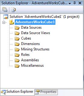
Figure 15-1: New Analysis Services project

Defining a Data Source

A data source provides the cube's connection to the staging tables, which the cube uses as source data. To define a data source, you'll use the Data Source Wizard. You can launch this wizard by right-clicking on the Data Sources folder in your new Analysis Services project. The wizard will walk you through the process of defining a data source for your cube, including choosing a connection and specifying security credentials to be used to connect to the data source.

Try It!

To define a data source for the new cube, follow these steps:

1. Right-click on the Data Sources folder in Solution Explorer and select New Data Source.
2. Read the first page of the Data Source Wizard and click Next.
3. You can base a data source on a new or an existing connection. Because you don't have any existing connections, click New.
4. In the Connection Manager dialog box, select the server containing your analysis services sample database from the Server Name combo box.
5. Fill in your authentication information.
6. Select the Native OLE DB\SQL Native Client provider (this is the default provider).
7. Select the AdventureWorksDW2008 database. Figure 15-2 shows the filled-in Connection Manager dialog box.



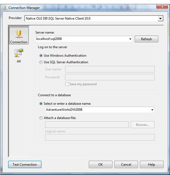
Figure 15-2: Setting up a connection


8. Click OK to dismiss the Connection Manager dialog box.
9. Click Next.
10. Select Use the Service Account impersonation information and click Next.
11. Accept the default data source name and click Finish.

Defining a Data Source View

A data source view is a persistent set of tables from a data source that supply the data for a particular cube. It lets you combine tables from as many data sources as necessary to pull together the data your cube needs. BIDS also includes a wizard for creating data source views, which you can invoke by right-clicking on the Data Source Views folder in Solution Explorer.

Try It!

To create a new data source view, follow these steps:

1. Right-click on the Data Source Views folder in Solution Explorer and select New Data Source View.
2. Read the first page of the Data Source View Wizard and click Next.
3. Select the Adventure Works DW data source and click Next. Note that you could also launch the Data Source Wizard from here by clicking New Data Source.
4. Select the FactFinance(dbo) table in the Available Objects list and click the > button to move it to the Included Object list. This will be the fact table in the new cube.
5. Click the Add Related Tables button to automatically add all of the tables that are directly related to the dbo.FactFinance table. These will be the dimension tables for the new cube. Figure 15-3 shows the wizard with all of the tables selected.





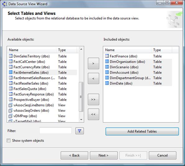
Figure 15-3: Selecting tables for the data source view


6. Click Next.
7. Name the new view Finance and click Finish. BIDS will automatically display the schema of the new data source view, as shown in Figure 15-4.

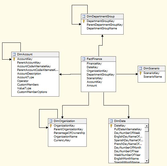
Figure 15-4: The Finance data source view

Invoking the Cube Wizard

As you can probably guess at this point, you invoke the Cube Wizard by right-clicking on the Cubes folder in Solution Explorer. The Cube Wizard interactively explores the structure of your data source view to identify the dimensions, levels, and measures in your cube.

Try It!

To create the new cube, follow these steps:

1. Right-click on the Cubes folder in Solution Explorer and select New Cube.
2. Read the first page of the Cube Wizard and click Next.
3. Select the option to Use Existing Tables.
4. Click Next.
5. The Finance data source view should be selected in the drop-down list at the top. Place a checkmark next to the FactFinance table to designate it as a measure group table and click Next.
6. Remove the check mark for the field FinanceKey, indicating that it is not a measure we wish to summarize, and click Next.
7. Leave all Dim tables selected as dimension tables, and click Next.
8. Name the new cube FinanceCube and click Finish.

Defining Dimensions

The cube wizard defines dimensions based upon your choices, but it doesn't populate the dimensions with attributes. You will need to edit each dimension, adding any attributes that your users will wish to use when querying your cube.

Try It!

1. In BIDS, double click on DimDate in the Solution Explorer.
2. Using Table 15-1 below as a guide, drag the listed columns from the right-hand panel (named Data Source View) and drop them in the left-hand panel (named Attributes) to include them in the dimension.
   
   

   DimDate

   CalendarYear

   CalendarQuarter

   MonthNumberOfYear

   DayNumberOfWeek

   DayNumberOfMonth

   DayNumberOfYear

   WeekNumberOfYear

   FiscalQuarter

   FiscalYear

   
   
   Table 15-1
   
   
3. Using Table 15-2, add the listed columns to the remaining four dimensions.
   
   

DimDepartmentGroup

DepartmentGroupName

DimAccount

AccountDescription

AccountType

DimScenario

ScenarioName

DimOrganization

OrganizationName

Table 15-2

Adding Dimensional Intelligence

One of the most common ways data gets summarized in a cube is by time. We want to query sales per month for the last fiscal year. We want to see production values year-to-date compared to last year's production values year-to-date. Cubes know a lot about time.

In order for SQL Server Analysis Services to be best able to answer these questions for you, it needs to know which of your dimensions stores the time information, and which fields in your time dimension correspond to what units of time. The Business Intelligence Wizard helps you specify this information in your cube.

Try It!

1. With your FinanceCube open in BIDS, click on the Business Intelligence Wizard button on the toolbar.
2. Read the initial page of the wizard and click Next.
3. Choose to Define Dimension Intelligence and click Next.
4. Choose DimDate as the dimension you wish to modify and click Next.
5. Choose Time as the dimension type. In the bottom half of this screen are listed the units of time for which cubes have knowledge. Using the Table 15-1 below, place a checkmark next to the listed units of time and then select which field in DimDate contains that type of data.
   
   

Time Property Name	Time Column
Year	CalendarYear
Quarter	CalendarQuarter
Month	MonthNumberOfYear
Day of Week	DayNumberOfWeek
Day of Month	DayNumberOfMonth
Day of Year	DayNumberOfYear
Week of Year	WeekNumberOfYear
Fiscal Quarter	FiscalQuarter
Fiscal Year	FiscalYear

Table 15-1:Time columns for FinanceCube

6. Click Next.

Hierarchies

You will also need to create hierarchies in your dimensions. Hierarchies are defined by a sequence of fields, and are often used to determine the rows or columns of a pivot table when querying a cube.

Try It!

1. In BIDS, double-click on DimDate in the solution explorer.
2. Create a new hierarchy by dragging the CalendarYear field from the left-hand pane (called Attributes) and drop it in the middle pane (called Hierarchies.)
3. Add a new level by dragging the CalendarQuarter field from the left-hand panel and drop it on the <new level> spot in the new hierarchy in the middle-panel.
4. Add a third level by dragging the MonthNumberOfYear field to the <new level> spot in the hierarchy.
5. Right-click on the hierarchy and rename it to Calendar.
6. Adding Dimensional IntelligenceIn the same manner, create a hierarchy named Fiscal that contains the fields FiscalYear, FiscalQuarter and MonthNumberOfYear. Figure 15-5 shows the hierarchy panel.

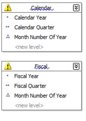
Figure 15-5: DimDate hierarchies

Deploying and Processing a Cube

At this point, you've defined the structure of the new cube - but there's still more work to be done. You still need to deploy this structure to an Analysis Services server and then process the cube to create the aggregates that make querying fast and easy.

To deploy the cube you just created, select Build > Deploy AdventureWorksCube1. This will deploy the cube to your local Analysis Server, and also process the cube, building the aggregates for you. BIDS will open the Deployment Progress window, as shown in Figure 15-5, to keep you informed during deployment and processing.

Try It!

To deploy and process your cube, follow these steps:

1. In BIDS, select Project > AdventureWorksCube1 from the menu system.
2. Choose the Deployment category of properties in the upper left-hand corner of the project properties dialog box.
3. Verify that the Server property lists your server name. If not, enter your server name. Click OK. Figure 15-6 shows the project properties window.



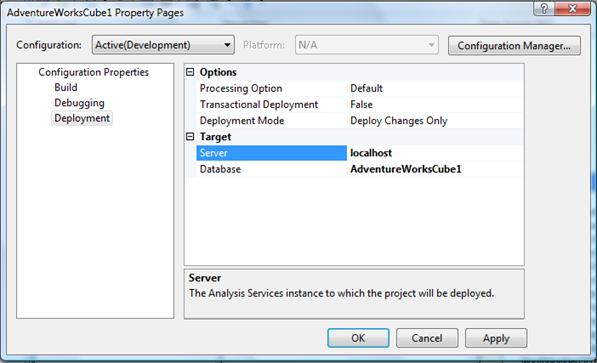
Figure 15-6: Project Properties

4. From the menu, select Build > Deploy AdventureWorksCube1. Figure 15-7 shows the Cube Deployment window after a successful deployment.

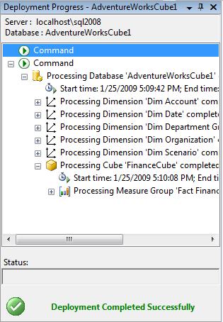
Figure 15-7: Deploying a cube

SSAS 2008 Tutorial: Exploring a Data Cube

At last you're ready to see what all the work was for. BIDS includes a built-in Cube Browser that lets you interactively explore the data in any cube that has been deployed and processed. To open the Cube Browser, right-click on the cube in Solution Explorer and select Browse. Figure 15-8 shows the default state of the Cube Browser after it's just been opened.

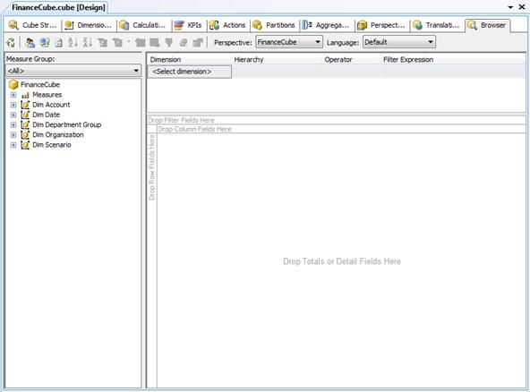
Figure 15-8: The cube browser in BIDS

The Cube Browser is a drag-and-drop environment. If you've worked with pivot tables in Microsoft Excel, you should have no trouble using the Cube browser. The pane to the left includes all of the measures and dimensions in your cube, and the pane to the right gives you drop targets for these measures and dimensions. Among other operations, you can:

• Drop a measure in the Totals/Detail area to see the aggregated data for that measure.
• Drop a dimension hierarchy or attribute in the Row Fields area to summarize by that value on rows.
• Drop a dimension hierarchy or attribute in the Column Fields area to summarize by that value on columns.
• Drop a dimension hierarchy or attribute in the Filter Fields area to enable filtering by members of that hierarchy or attribute.
• Use the controls at the top of the report area to select additional filtering expressions.

Try It!

To see the data in the cube you just created, follow these steps:

1. Right-click on the cube in Solution Explorer and select Browse.
2. Expand the Measures node in the metadata panel (the area at the left of the user interface).
3. Expand the Fact Finance measure group.
4. Drag the Amount measure and drop it on the Totals/Detail area.
5. Expand the Dim Account node in the metadata panel.
6. Drag the Account Description attribute and drop it on the Row Fields area.
7. Expand the Dim Date node in the metadata panel.
8. Drag the Calendar hierarchy and drop it on the Column Fields area.
9. Click the + sign next to year 2001 and then the + sign next to quarter 3.
10. Expand the Dim Scenario node in the metadata panel.
11. Drag the Scenario Name attribute and drop it on the Filter Fields area.
12. Click the dropdown arrow next to scenario name. Uncheck all of the checkboxes except for the one next to the Budget value.

Figure 15-9 shows the result. The Cube Browser displays month-by-month budgets by account for the third quarter of 2001. Although you could have written queries to extract this information from the original source data, it's much easier to let Analysis Services do the heavy lifting for you.

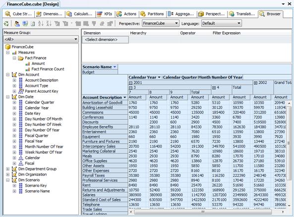
Figure 15-9: Exploring cube data in the cube browser

SSAS 2008 Tutorial: Exercises

Although cubes are not typically created with such a single purpose in mind, your task is to create a data cube, based on the data in the AdventureWorksDW2008 sample database, to answer the following question: what were the internet sales by country and product name for married customers only?

Solutions to Exercises

To create the cube, follow these steps:

1. Select Microsoft SQL Server 2008 „ SQL Server Business Intelligence Development Studio from the Programs menu to launch Business Intelligence Development Studio.
2. Select File > New > Project.
3. In the New Project dialog box, select the Business Intelligence Projects project type.
4. Select the Analysis Services Project template.
5. Name the new project AdventureWorksCube2 and select a convenient location to save it.
6. Click OK to create the new project.
7. Right-click on the Data Sources folder in Solution Explorer and select New Data Source.
8. Read the first page of the Data Source Wizard and click Next.
9. Select the existing connection to the AdventureWorksDW2008 database and click Next.
10. Select Service Account and click Next.
11. Accept the default data source name and click Finish.
12. Right-click on the Data Source Views folder in Solution Explorer and select New Data Source View.
13. Read the first page of the Data Source View Wizard and click Next.
14. Select the Adventure Works DW2008 data source and click Next.
15. Select the FactInternetSales(dbo) table in the Available Objects list and click the > button to move it to the Included Object list.
16. Click the Add Related Tables button to automatically add all of the tables that are directly related to the dbo.FactInternetSales table. Also add the DimGeography dimension.
17. Click Next.
18. Name the new view InternetSales and click Finish.
19. Right-click on the Cubes folder in Solution Explorer and select New Cube.
20. Read the first page of the Cube Wizard and click Next.
21. Select the option to Use Existing Tables.
22. Select FactInternetSales and FactInternetSalesReason tables as the Measure Group Tables and click Next.
23. Leave all measures selected and click Next.
24. Leave all dimensions selected and click Next.
25. Name the new cube InternetSalesCube and click Finish.
26. In the Solution Explorer, double click the DimCustomer dimension.
27. Add the MaritalStaus field as an attribute, along with any other fields desired.
28. Similarly, edit the DimSalesTerritory dimension, adding the SalesTerritoryCountry field along with any other desired fields.
29. Also edit the DimProduct dimension, adding the EnglishProductName field along with any other desired fields.
30. Select Project > AdventureWorksCube2 Properties and verify that your server name is correctly listed. Click OK.
31. Select Build > Deploy AdventureWorksCube2.
32. Right-click on the cube in Solution Explorer and select Browse.
33. Expand the Measures node in the metadata panel.
34. Drag the Order Quantity and Sales Amount measures and drop it on the Totals/Detail area.
35. Expand the Dim Sales Territory node in the metadata panel.
36. Drag the Sales Territory Country property and drop it on the Row Fields area.
37. Expand the Dim Product node in the metadata panel.
38. Drag the English Product Name property and drop it on the Column Fields area.
39. Expand the Dim Customer node in the metadata panel.
40. Drag the Marital Status property and drop it on the Filter Fields area.
41. Click the dropdown arrow next to Marital Status. Uncheck the S checkbox.

Figure 15-10 shows the finished cube.

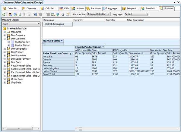
Figure 15-10: The AdventureWorksCube2 cube