Tired of your fellow humans being probed by aliens? It’s time to probe back! Well, at least, probe the data on UFO sightings. To do this, we’ll show-case one of the most popular open source tools for analyzing data: the pandas package.
Not to be confused with the Chinese bear, the name pandas is a portmanteau of panel data, an econometrics term for multidimensional structured datasets. As a package for the popular programming language, Python, the project arose in response to a number of key issues the language had with handling data. Its author, Wes McKinney, noted that base Python did not cope gracefully with missing data, time series, labeling of data and metadata and common merge/join operations found in comparable analysis tools, such as SAS, R, SQL and Matlab. The project began in 2008 and is an open-source project with enthusiastic support.
Consequently, pandas usage has grown steadily, becoming one of the most popular and powerful tools in a Data Scientist’s workshop1. It provides a versatile framework for plenitudinous tasks in data science, designed to easily import, manipulate and present data efficiently and (mostly) intuitively. When teaching how to use pandas in one of our Data Science courses, we recommend Python for Data Science Handbook by Jake VanderPlas. I also highly recommend Wes McKinney’s Python for Data Analysis (both published by O’Reilly media).
Two key structures are introduced with pandas: the DataFrame and the Series objects. The former will be familiar to those with experience using the R language for statistical computing (as data.frame); it was indeed the prototype for the pandas version. A Series is a one-dimensional array, with optional labeling and naming. In many ways, a Series acts like a vector, in that common vector operations are defined if the elements are numerical types.
However, it can be referenced by label, similar to a dictionary, and it also supports time series relatively gracefully. A DataFrame is a two-dimensional tabular data structure of one or more Series objects, with labels for each axis: rows and columns.
So, without further ado, let’s get our probes ready, and analyze some data!
The National UFO Reporting Center
The National UFO Reporting Center (NUFORC) hosts and curates a comprehensive repository of UFO sightings. Physically housed in Missile Site #6 — an abandoned Atlas missile bunker (of course) in rural Washington state — NUFORC is currently directed by Peter Davenport, who took the helm in 1994. Members of the public may report a possible UFO experience via the website, fax or telephone. Care is taken to ascertain whether reports are potential hoaxes or otherwise erroneous.
The reports themselves are publicly accessible via the NUFORC website. On an ordered collection of web pages, the entries are stored as plain HTML tables, where each observation is a single line. The columns contain data on the event date, city and US state (where applicable), shape of the object(s) witnessed, duration of the event, a brief summary text, and, finally, the date the report was posted to NUFORC. Typical entries look like the following:
Two Diamond shaped craft spotted over southern Maryland
7/5/05
As you can probably guess, the entries make for a fun and interesting read.
For the purposes of analysis, I generated a single Comma Separated Variable (CSV) file from the pages using a web-scraper2 constructed using the excellent scrapy Python package3. One important function of the web scraper was to capture more accurate times for events. Many of the earlier date/time entries only had two digits for the year (yy), yet the archive extends from the fifteenth century to now (September 2018). This meant that most (all?) of the reports from, e.g. 1967, appear as 2067 etc. However, thanks to the curation efforts of NUFORC, the year and month are held as six-digit metadata in the URL for the entries; this vital information is parsed4 and added to each entry.
1: Check Your Data
First of all, whenever possible, you should briefly examine the data before importing it, with a text editor or viewer. I prefer the excellent file pager less, which is perfect for examining large files without crashing or noticeably slowing your personal computer.
Good. Looks like a CSV file should, complete with comma delimiters and a header line.
Note the ‘year’ and ‘month’ fields were extracted directly from the URL (which is a different URL to the summary links provided in the table). The ‘summary’ field was omitted because it’s a truncated version of what is contained in the ‘url,’ and there’s not much we can do, in terms of analysis, for now anyway (that is the domain of Natural Language Processing).
If you have not already installed the pandas library, do so now. We recommend using
Anaconda’s conda package manager, to keep versions consistent. However, you could also use pip (pip install pandas) or Easy Install (easy_install pandas).
Import this, as well as the popular graphics package, matplotlib:
import pandas as pd
import matplotlib as mpl
Let’s tweak some of the plotting defaults for some flavor (note that you probably will not have the Souvenir font installed on your local system):
2: Beam Me Up: Import the Data and Have a Look Around
Importing data files with pandas is very easy. We have stored our UFO Reports data in a Comma Separated Variable (CSV) file (national_ufo_reports.csv), so we can simply use the .read_csv() method:
ufo_df = pd.read_csv("national_ufo_reports.csv")
A somewhat common practice is to put a _df at the end of a variable name to remind us that it is a DataFrame object (recall that a DataFrame is a collection of Series objects). Our UFO data is in what is often referred to as a ‘wide’ table format, where each column is a variable, and each row an observation.
It is a simple matter to interrogate the first few elements using the .head() method associated with pandas DataFrames:
ufo_df.head(5)

   date_time      year    month  city         state shape
duration  posted  url
   0  8/30/18 22:00 2018        8  Morehead City  NC    Unknown
1 hour 8/31/18  http://www.nuforc.org/webreports/142/S142925.html
   1  8/30/18 21:36 2018  8   Commerce        GA    Circle
5 seconds  8/31/18 http://www.nuforc.org/webreports/142/S142924.html
   2  8/30/18 21:15 2018  8   Queens Village  NY    Light
15 minutes  8/31/18 http://www.nuforc.org/webreports/142/S142929.html
   3  8/30/18 20:48 2018  8   Independence    KS    Unknown
3 minutes  8/31/18 http://www.nuforc.org/webreports/142/S142928.html
   4  8/30/18 20:25 2018  8   Redding         CA    Light
5 seconds  8/31/18 http://www.nuforc.org/webreports/142/S142926.html
Note the row indices (here, 0—5) and column labels (‘date_time’—’url’). We can easily call any given element. We can look at the Series from any column by directly calling it with [] (note the use of .head() here to suppress the otherwise large number of rows):
Note the default for .head() is the first five rows.
We could look at the fourth row (index of 3 because, as conventional in Python, we index from 0) by using .loc[]:
ufo_df.loc[3]

date_time         8/30/18 20:48
year                       2018
month                         8
city               Independence
state                        KS
shape                   Unknown
duration              3 minutes
posted                  8/31/18
url     http://www.nuforc.org/webreports/142/S142928.html
Name:   3, dtype: object
Because any given contiguous region of a data file tends to have localized observations, it pays to take a random sample of a DataFrame to better gauge the general variability of the dataset. To take five such random samples:
NOTE: If you look in the help documentation ( help(pd.DataFrame.loc) ) you’ll notice something of an apology: “note that contrary to usual python slices, **both** the start and the stop are included!”
If you prefer to use numbers instead of labels, use .iloc[] instead:
ufo_df.iloc[0:5, 6:9]
Confusingly, .iloc[] slices with the conventional start and stop indices. Also note, for both slicing methods, square brackets [] are used instead of parentheses ().
3: The Operating Table: Initial Exploratory Data Analysis
The following are typical steps for Exploratory Data Analysis (EDA) of a dataset, once the data are imported.
Size and scope of the data
What are the dimensions of the DataFrame?
ufo_df.shape

(115877, 9)
Around 116,000 rows and 9 columns.
We could just as easily have found the number of rows by using the built-in Python len() function:
len(ufo_df) # 115877
What sort of data is each column?
ufo_df.dtypes

date_time    object
year          int64
month         int64
city         object
state        object
shape        object
duration     object
posted       object
url          object
dtype: object
Confusingly, ‘object’ here refers to strings as well as other possible objects. How do the numeric data vary (range, median, mean)?
ufo_df.describe()

                 year            month
count   115877.000000  115877.000000
mean      2006.127687       6.850945
std         11.481973         3.216381
min       1400.000000         1.000000
25%       2003.000000         4.000000
50%       2009.000000       7.000000
75%       2013.000000       9.000000
max       2018.000000        12.000000
Half of all observations in this dataset were from 2009 until now (September 2018). How much data is missing?
ufo_df.isnull().sum()
Note the ‘chaining’ of methods here, with the .sum() operating on the result of the .isnull()
operation. This powerful concept will be used throughout the remainder of this tutorial.
date_time    0
year         0
month        0
city       227
state     8438
shape     3686
duration  3896
posted       0
url          0
dtype: int64
None of the date-like entries are missing, as too for the URLs.
The duration and shape may not be well defined or known, so the ~4,000 missing for each is understandable, at 3% of the observations. The state is not defined for most non-US entries, and there are plenty of those. In this rare case, there is no need for imputation5 — for now. Great!
Filtering and Initial Data Cleaning
Do we need to filter by year?
The dates prior to 1900 are likely to be based on heavy, retrospective, speculation, or worse: errors due to data entry!
Filtering is simple in pandas. We can easily filter the ‘year’ field by evaluating a logical Series:
ufo_df[ufo_df['year'] < 1900].count() # 24
There is also the .query() method to achieve a similar effect (although this performs better with larger datasets):
ufo_df.query('year<1900').count() # 24
So there are only 24 such observations before 1900. Upon manual inspection, only three of these entries are mis-entered. This is an unexpected bonus!
For example, one entry was dated as the year 1721, when it was obviously a replication of the time (21:30) with the yy year format (17, for 2017). Otherwise, this is unexpectedly nice data!
We have officially entered the data cleaning stage (often referred to as ‘data wrangling,’ or ‘data munging’). For realistic datasets, this process generally occupies an inordinate amount of time.
Let’s remove the bad dates for the single entries in years 1617, 1615 and 1721. We can create a tiny DataFrame of them:
…or you could have indexed from the bad_dates DataFrame:
ufo_df.drop(index=bad_dates.index, inplace=True)
Note the .drop() method has a convenient inplace option, so you don’t need to update a copy of the DataFrame.
Whenever you perform data wrangling and cleaning, it is good policy to check you performed the operation correctly.
ufo_df.shape

(115874, 9)
OK, good. Three fewer rows, correct number of columns.
Dates and Time-series
As with most analysis frameworks, dates are a special class unto themselves. This is because everyone has a different way of writing them (for example, a European may write 4 July 2018 as 4/7/2018, while an American might write 7/4/2018), and there are so many things you want to do with them.
Here, we explicitly force the ‘date_time’ column to be a DateTime object:
ufo_df.dtypes[0:4]

date_time    datetime64[ns]
year                  int64
month                 int64
city                 object
dtype: object
NOTE: This makes use of the default format specifications, including dayfirst=False and yearfirst=False. This is because the NUFORC database follows the American convention. Don’t always expect this.
If we already expect a date format upon import, there is an option to specify a date-time column, so we could have done this right at the import phase, i.e.:
However, as mentioned earlier this particular dataset is tricky! The date_time input wraps around the year, so will not give the correct century in many cases.
As mentioned above, the dataset we use has already parsed the ‘proper’ year and month from the URL itself, because we had anticipated this very issue (see the description on the Spider used to obtain this data from the NUFORC website).
The topic of the time-series analysis capabilities of pandas, including resampling and windowing, could be a whole tutorial itself. But we shall leave it at this for the time being.
4: Graphical Analysis
Pandas has support for a wide range of graphical analysis. These are really a number of wrappers to the matplotlib.pyplot Python library.
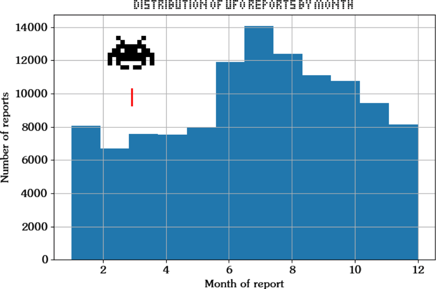
Let’s analyze the univariate distribution of observations by month:
ufo_df['month'].hist(bins=12)
Because the plotting functions are wrappers for matplotlib, you can add attributes to the figures accordingly:
import matplotlib.pyplot as plt

plt.xlabel("Month of report")
plt.ylabel("Number of reports")
plt.title("Distribution of UFO reports by month")
You can save the plot like any matplotlib figure:
plt.savefig("UFO_observations_by_month.png")
Or you could examine it interactively with:
plt.show()
Note that the object is ‘used’ up by saving or displaying6.
It appears that summer (in the Northern Hemisphere) is the time to spot UFOs. It makes sense!
Hopefully you have seen here some of the great power offered by the pandas framework. The process of importation, through the exploration and cleaning and basic wrangling of data, is but a simple matter. Time series, handling missing data and subsequent visualization of the results may be simply performed in a single line!
But what about the more sophisticated tools, such as grouping, aggregation joining advanced string methods and other functions? Are they just as simple to carry out too? We’re talking grouping, aggregation and joining data, as well as other powerful functions.
For that—you’ll have to tune in for the next installment, where we visit the Mother Ship!
1 In fact you can find three articles using pandas, with different applications, on this very site: [1], [2] & [3]
2 Often referred to as a ‘spider’. Because it, y’know, crawls the web.
3 The details of which would comprise its own article, but you may download the code from here.
4 No, this isn’t a typo of ‘passed.’ This is a technical term for ‘interpreting some output’.
5 A fancy, ten-dollar, word for ‘figuring out how to handle missing data’. It has the same Latin roots as for ‘input,’ and is similar to that for ‘amputation’ (which is roughly ‘to clean by cutting back’).
Ra is originally from New Zealand, has a PhD in physics, is a data scientist, and has taught for Accelebrate in the US and in Africa. His specialties are R Programming and Python.